Mar 09, 2009
Originally posted on Half an Hour, March 9, 2009.
The Network Phenomenon: Empiricism and the New Connectionism
Stephen Downes, 1990
(The whole document in MS-Word)
TNP Part III Previous Post
IV. Connectionism
A. Basic Connectionist Structures
A connectionist system consists of a set of neurons, or "units", and a set of connections between those units. The units may be activated or inactivated, Most systems employ simple on-off activations, although other systems allow for degrees of activation. The motivation for this basic structure is biological. Connectionist systems emulate human brains, and human brains consist of interconnected neurons which may be activated (spiking) or inactivated.
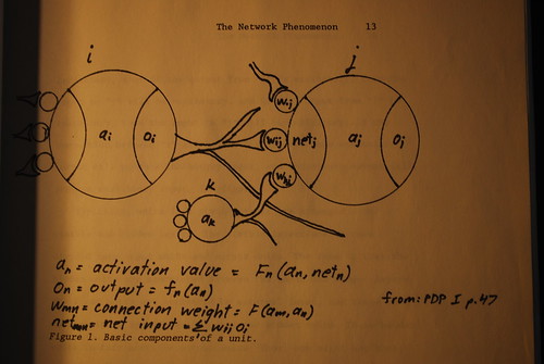
The idea is that a unit "i", if activated, sends signals or "output" via connections to other units. Other units, in turn, send signals to other units, including unit "i". These signals comprise part of the "input" to "i". It is also possible to provide input to "i" via some external mechanism, in which case the input is referred to as "external input". For any given unit "i", the state of activation of "i" at time t depends on its external and internal input at time t and the state of activation at time t-1. Input can be excitatory or inhibitory. If it is excitatory, then the unit tends to become activated, while if it is inhibitory, then the unit tends to become inactivated.
Connections between units may similarly be excitatory or inhibitory. If a connection between two units "i" and "j" is excitatory, then if the output from "i: is excitatory, then the input to "j" will be excitatory, and if the output from "i" is inhibitory, then the input to "j" will be inhibitory. If the connection between "i" and "j" is inhibitory, then excitatory output will produce inhibitory input, and inhibitory output will produce excitatory input. See figure 1.
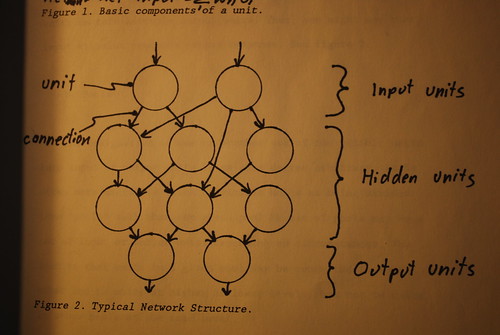
Typically, units in a given network are arranged into visible and hidden layers. The visible layers are in turn divided into input and output units. The idea is that the hidden units are sandwiched between the input and the output layers. The input units are activated by external input, and these in turn activate appropriately connected hidden units. These hidden units in turn activate output units. Thus, one might say that input stimulus produces output response. See figure 2.
b. Pools
The designation of one or another set of the visible units into input or output units is to some degree arbitrary. It is often more useful to think of visible units as being divided into "pools" such that any given pool or set of pools may be a set of input or output units depending on circumstances. The idea is that units in a given pool may be connected to each other and to units at higher or lower levels, but not to units in other pools at the same level.
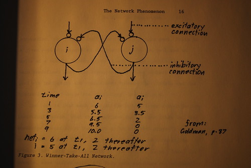
The basic idea is derived from Feldman. [12] Suppose we have two units "i" and "j", each with a single input and a single output. Excitatory input will activate the unit and it will in turn send excitatory output. Suppose now that each unit is connected to the other such that if "i" is activated, it will tend to inhibit "j", and if "j" is activated, it will tend to inhibit "i". Then over time, whichever unit re3ceives more input activation will tend toward maximum activation, while the other will tend toward minimum activation (that is, maximum inhibition). A network like this is called a "Winner-take all (WTA)" network. See figure 3.
If you do this with two or more units, you have a pool. An example of this sort of structure is McClelland and Rumelhart's "IAC (Interactive Activation and Competition)" network. [13] This is an interesting network because it shows how networks can categorize and generalize.
McClelland and Rumelhart use as an example a network called "Jets and Sharks". Each unit at the visible level stands for some property of a person, for example, his age (in20s, in30s, in40s), his occupation (burglar, pusher, etc.), his name, his education, and so on. Each of these sets of properties (age, occupation, name, education) constitutes a single pool. Units in a given pool are connected to other units in the pool and to units in a second, hidden layer of units. the connections have been predefined such that connections between members of a given pool are inhibitory and connections between the visible and the hidden layers of units are excitatory. See figure 4.
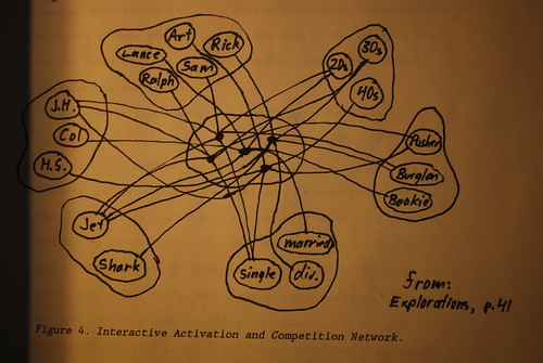
The idea is that each unit at the hidden layer stands for an individual person. What characterizes that person (that is, the knowledge stored about the person) is not some property of the unit in the hidden layer, but rather, the set of connections between that unit and the units at the visible layer. Take, for example, some hidden unit "i". This unit contains no information about the person. However, it is connected to the units at the visible layer standing for Jake, burglar, in20s, high school, Jet (the gang name), etc.
Suppose now that the network could learn the connections just described. Then it would have leaned a system of categorization. Each of the pools constitutes a distinct category. The fact that it i a category is established by the inhibitory connections between all and only units of a given pool and by the fact that one, and only one, unit in a given pool is connected to any given unit at the hidden layer. What makes, say, in20s, in30s, and in40s a single category is first the fact that they have something in common - they are all associated with some person - and second that they are mutually exclusive. The activation of one inhibits the rest.
The IAC network can perform a number of associative and inductive tasks. For example, suppose we activated "burglar", "in20s" and "high school". Then, because of the excitatory connections to a given hidden unit, that unit would become activated. In turn, the hidden unit would send excitatory output via an excitatory connection to the visible unit representing "Jake". Thus, by input to a set of features, an individual's name may be recognized. What is interesting is that the name may be activated even if the description is incomplete or incorrect. [14] The reliability of such a conclusion drawn in such circumstances varies according to the scale of the missing or incorrect information and according to other connections in the network.
Such a network can also generlaize. For example, suppose the unit for "Jet" were activated. This unit is connected to a number of hidden units, and these will be activated. Each of the hidden units will send excitatory output to units in the other visible pools. Several units in each pool may be excited. However, since the connections between the units of a given [pool] are inhibitory, then only the unit with the greatest excitatory input will be activated; the rest will be inhibited, Thus, upon the activation of "Jets", a set of units, one in each pool, will also become activated. This set of units is a "stereotypical" picture of the Jets. For example, activating "Jets" may result in the activation of "in20s", "pusher", "high school", etc. One might say that these features constitute a definition of the category "Jets" even though no individual Jet has all and only those stereotypical features.
A similar sort of network performs well in visual recognition or multiple constraint tasks. One could input observed features of a person at a distance and the output could be that person's name. As with the previous example, the nature and reliability of the conclusion will vary according to circumstances. For example, a distinctive walk could very quickly aid in the determination of a given person's name, but if the system has information about two such people with the same distinctive walk, then this determination will not be so quick and so sure.
C. Learning in Connectionist Networks
In my mind, the real advantage of connectionism does not lie in the features just described, for those features could be realized by a system with enough predefined rules. Rather, the advantage is that such a system can learn its own connective structure. A network learns by adjusting connection w3eights between different units. There are several ways of doing this, and this accounts for one of the major differences between types of connectionist systems.
The simplest sort of system employs the Hebb rule. According to the Hebb rule, if two units are simultaneously activated, then the connection between thm should b strengthened. Similarly, the connection between two units should be strengthened if the two units are simultaneously inhibited. If the two units are at a given time at different states of activation (one is excited, the other inhibited) then the connection is weakened. The major problem (in my mind) with the Hebb rule is that it doesn't work in networks with more than two layers. This is a substantial weakness, since as Minsky and Papert point out, a two-layer network cannot distinguish between, say, exclusive and inclusive disjunctions. [15]
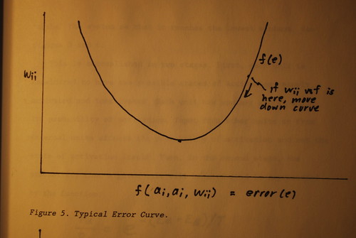
Most contempoary systems use a version of the "delta-learning rule". In such a system it is important to distinguish between input and output units. Input units are excited and consequent output noted (if there are more than two layers and no connections are yet established there will be no output at first). The output obtained is compared to the desired output and an error is computed. From this error a correction can be calculated (take the error and apply a linear or non-linear function to it. This produces a curve, the slope of which will be zero at the point of minimum error. There are various strategies for going 'down' the curve.) This correction is then propagated back through the network and the correction is distributed across the connections which contributed to the error. This process is called back-propagation.
Such a system depends on a teacher. This sometimes seems to pose a problem for artificial intelligence theorists who would rather the machine learned completely on its own. [16] However, experience can teach. The concept of "lessons of nature" dates back at least to the Scholastic philosophy of the middle ages and is a central thesis of empiricism. One can imagine how some particular output (a response or behaviour) might require correction because it causes, or fails to prevent, pain.
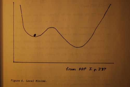
One of the dificulties encountered in back=propagation systems is the problem of the "local minima". What happens when you calculate the error curve for a number of variables is that you might not get one single location where the curv is zero; you might get several. One such point may be still an error, but since the slope i zero, there is no means for the system to correct itself, since the degree of correction is usually a function of the slope of the curve. What you want to do is to "shake" the system so that it reaches the lowest minimum. See figures 5 and 6.
This is accomplished in two stages. First, each unit is considered to have two possible states of activation, namely, activated and inactivated. Each unit has another state, which is its probability of activation. Input from other units or from external units affects the probability of activation and not the state of activation itself. Then, in the second stage, the probability that a given nit will be activated is represented by the function:
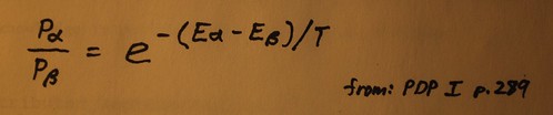
where E stands for the "energy" of the system and "T" stands for the "temperature" of the system. [17]
The reason why the terms "energy" and "temperature" are employed is that the equation above is borrowed directly from physics. Essentially, the higher the temperature, the more random the activation or inactivation of a given unit will be. As it turns out, if a system is started at a high temperature and then, as processing continues, the temperature is lowered, the system is much less likely to settle into a local minimum. This process is called "annealing" and is exactly analagous to the physical process (used to produce stable crystalline formations) of the same name.
There are several useful features of this process which I won't detail, however, I will mention that these is an equation such that the energy (and hence, error) of any given connection can be determined. Hence, energy minimization (and hence, error correction) can be accomplished at a local level, with no regard to the global properties of a system. This means that "higher level" knowledge is not required for error correction.
TNP Part V Next Post
[12] Feldman, J.A. and D.H. Ballard, "Connectionist Models and Their Properties", Cognitive Science 6 (1982), pp. 205-254; cited in Alvin Goldman, "Epistemology and the New Connectionism", in N. Garver and P. Hare, Naturalism and Rationality (1986), p. 84.
[13] Parallel Distributed Processing I, p. 28.
[14] This is called content addressability and differs from traditional systems. See James Anderson and Geoffrey Hinton, "Models of Information Processing in the Brain", in Anderson and Hinton, editors, Parallel Models of Associative Memory, p.11.
[15] Marvin Minsky and Seymour Papert, Perceptrons.
[16] Eg., Hinton, who proposed that learning could be accomplished without training if the system had a built-in coherence requirement. Geoffrey Hinton, "The Social Construction of Objective Reality in a neural Network". Connectionism conference, Simon Fraser University, 1990.
[17] This equation is specific to "Boltzmann" machine versions; there are other equations that accomplish the same thing. These are described in Parallel Distributed Processing I, ch. 6 and 7.
The Network Phenomenon: Empiricism and the New Connectionism
Stephen Downes, 1990
(The whole document in MS-Word)
TNP Part III Previous Post
IV. Connectionism
A. Basic Connectionist Structures
A connectionist system consists of a set of neurons, or "units", and a set of connections between those units. The units may be activated or inactivated, Most systems employ simple on-off activations, although other systems allow for degrees of activation. The motivation for this basic structure is biological. Connectionist systems emulate human brains, and human brains consist of interconnected neurons which may be activated (spiking) or inactivated.
The idea is that a unit "i", if activated, sends signals or "output" via connections to other units. Other units, in turn, send signals to other units, including unit "i". These signals comprise part of the "input" to "i". It is also possible to provide input to "i" via some external mechanism, in which case the input is referred to as "external input". For any given unit "i", the state of activation of "i" at time t depends on its external and internal input at time t and the state of activation at time t-1. Input can be excitatory or inhibitory. If it is excitatory, then the unit tends to become activated, while if it is inhibitory, then the unit tends to become inactivated.
Connections between units may similarly be excitatory or inhibitory. If a connection between two units "i" and "j" is excitatory, then if the output from "i: is excitatory, then the input to "j" will be excitatory, and if the output from "i" is inhibitory, then the input to "j" will be inhibitory. If the connection between "i" and "j" is inhibitory, then excitatory output will produce inhibitory input, and inhibitory output will produce excitatory input. See figure 1.
Typically, units in a given network are arranged into visible and hidden layers. The visible layers are in turn divided into input and output units. The idea is that the hidden units are sandwiched between the input and the output layers. The input units are activated by external input, and these in turn activate appropriately connected hidden units. These hidden units in turn activate output units. Thus, one might say that input stimulus produces output response. See figure 2.
b. Pools
The designation of one or another set of the visible units into input or output units is to some degree arbitrary. It is often more useful to think of visible units as being divided into "pools" such that any given pool or set of pools may be a set of input or output units depending on circumstances. The idea is that units in a given pool may be connected to each other and to units at higher or lower levels, but not to units in other pools at the same level.
The basic idea is derived from Feldman. [12] Suppose we have two units "i" and "j", each with a single input and a single output. Excitatory input will activate the unit and it will in turn send excitatory output. Suppose now that each unit is connected to the other such that if "i" is activated, it will tend to inhibit "j", and if "j" is activated, it will tend to inhibit "i". Then over time, whichever unit re3ceives more input activation will tend toward maximum activation, while the other will tend toward minimum activation (that is, maximum inhibition). A network like this is called a "Winner-take all (WTA)" network. See figure 3.
If you do this with two or more units, you have a pool. An example of this sort of structure is McClelland and Rumelhart's "IAC (Interactive Activation and Competition)" network. [13] This is an interesting network because it shows how networks can categorize and generalize.
McClelland and Rumelhart use as an example a network called "Jets and Sharks". Each unit at the visible level stands for some property of a person, for example, his age (in20s, in30s, in40s), his occupation (burglar, pusher, etc.), his name, his education, and so on. Each of these sets of properties (age, occupation, name, education) constitutes a single pool. Units in a given pool are connected to other units in the pool and to units in a second, hidden layer of units. the connections have been predefined such that connections between members of a given pool are inhibitory and connections between the visible and the hidden layers of units are excitatory. See figure 4.
The idea is that each unit at the hidden layer stands for an individual person. What characterizes that person (that is, the knowledge stored about the person) is not some property of the unit in the hidden layer, but rather, the set of connections between that unit and the units at the visible layer. Take, for example, some hidden unit "i". This unit contains no information about the person. However, it is connected to the units at the visible layer standing for Jake, burglar, in20s, high school, Jet (the gang name), etc.
Suppose now that the network could learn the connections just described. Then it would have leaned a system of categorization. Each of the pools constitutes a distinct category. The fact that it i a category is established by the inhibitory connections between all and only units of a given pool and by the fact that one, and only one, unit in a given pool is connected to any given unit at the hidden layer. What makes, say, in20s, in30s, and in40s a single category is first the fact that they have something in common - they are all associated with some person - and second that they are mutually exclusive. The activation of one inhibits the rest.
The IAC network can perform a number of associative and inductive tasks. For example, suppose we activated "burglar", "in20s" and "high school". Then, because of the excitatory connections to a given hidden unit, that unit would become activated. In turn, the hidden unit would send excitatory output via an excitatory connection to the visible unit representing "Jake". Thus, by input to a set of features, an individual's name may be recognized. What is interesting is that the name may be activated even if the description is incomplete or incorrect. [14] The reliability of such a conclusion drawn in such circumstances varies according to the scale of the missing or incorrect information and according to other connections in the network.
Such a network can also generlaize. For example, suppose the unit for "Jet" were activated. This unit is connected to a number of hidden units, and these will be activated. Each of the hidden units will send excitatory output to units in the other visible pools. Several units in each pool may be excited. However, since the connections between the units of a given [pool] are inhibitory, then only the unit with the greatest excitatory input will be activated; the rest will be inhibited, Thus, upon the activation of "Jets", a set of units, one in each pool, will also become activated. This set of units is a "stereotypical" picture of the Jets. For example, activating "Jets" may result in the activation of "in20s", "pusher", "high school", etc. One might say that these features constitute a definition of the category "Jets" even though no individual Jet has all and only those stereotypical features.
A similar sort of network performs well in visual recognition or multiple constraint tasks. One could input observed features of a person at a distance and the output could be that person's name. As with the previous example, the nature and reliability of the conclusion will vary according to circumstances. For example, a distinctive walk could very quickly aid in the determination of a given person's name, but if the system has information about two such people with the same distinctive walk, then this determination will not be so quick and so sure.
C. Learning in Connectionist Networks
In my mind, the real advantage of connectionism does not lie in the features just described, for those features could be realized by a system with enough predefined rules. Rather, the advantage is that such a system can learn its own connective structure. A network learns by adjusting connection w3eights between different units. There are several ways of doing this, and this accounts for one of the major differences between types of connectionist systems.
The simplest sort of system employs the Hebb rule. According to the Hebb rule, if two units are simultaneously activated, then the connection between thm should b strengthened. Similarly, the connection between two units should be strengthened if the two units are simultaneously inhibited. If the two units are at a given time at different states of activation (one is excited, the other inhibited) then the connection is weakened. The major problem (in my mind) with the Hebb rule is that it doesn't work in networks with more than two layers. This is a substantial weakness, since as Minsky and Papert point out, a two-layer network cannot distinguish between, say, exclusive and inclusive disjunctions. [15]
Most contempoary systems use a version of the "delta-learning rule". In such a system it is important to distinguish between input and output units. Input units are excited and consequent output noted (if there are more than two layers and no connections are yet established there will be no output at first). The output obtained is compared to the desired output and an error is computed. From this error a correction can be calculated (take the error and apply a linear or non-linear function to it. This produces a curve, the slope of which will be zero at the point of minimum error. There are various strategies for going 'down' the curve.) This correction is then propagated back through the network and the correction is distributed across the connections which contributed to the error. This process is called back-propagation.
Such a system depends on a teacher. This sometimes seems to pose a problem for artificial intelligence theorists who would rather the machine learned completely on its own. [16] However, experience can teach. The concept of "lessons of nature" dates back at least to the Scholastic philosophy of the middle ages and is a central thesis of empiricism. One can imagine how some particular output (a response or behaviour) might require correction because it causes, or fails to prevent, pain.
One of the dificulties encountered in back=propagation systems is the problem of the "local minima". What happens when you calculate the error curve for a number of variables is that you might not get one single location where the curv is zero; you might get several. One such point may be still an error, but since the slope i zero, there is no means for the system to correct itself, since the degree of correction is usually a function of the slope of the curve. What you want to do is to "shake" the system so that it reaches the lowest minimum. See figures 5 and 6.
This is accomplished in two stages. First, each unit is considered to have two possible states of activation, namely, activated and inactivated. Each unit has another state, which is its probability of activation. Input from other units or from external units affects the probability of activation and not the state of activation itself. Then, in the second stage, the probability that a given nit will be activated is represented by the function:
where E stands for the "energy" of the system and "T" stands for the "temperature" of the system. [17]
The reason why the terms "energy" and "temperature" are employed is that the equation above is borrowed directly from physics. Essentially, the higher the temperature, the more random the activation or inactivation of a given unit will be. As it turns out, if a system is started at a high temperature and then, as processing continues, the temperature is lowered, the system is much less likely to settle into a local minimum. This process is called "annealing" and is exactly analagous to the physical process (used to produce stable crystalline formations) of the same name.
There are several useful features of this process which I won't detail, however, I will mention that these is an equation such that the energy (and hence, error) of any given connection can be determined. Hence, energy minimization (and hence, error correction) can be accomplished at a local level, with no regard to the global properties of a system. This means that "higher level" knowledge is not required for error correction.
TNP Part V Next Post
[12] Feldman, J.A. and D.H. Ballard, "Connectionist Models and Their Properties", Cognitive Science 6 (1982), pp. 205-254; cited in Alvin Goldman, "Epistemology and the New Connectionism", in N. Garver and P. Hare, Naturalism and Rationality (1986), p. 84.
[13] Parallel Distributed Processing I, p. 28.
[14] This is called content addressability and differs from traditional systems. See James Anderson and Geoffrey Hinton, "Models of Information Processing in the Brain", in Anderson and Hinton, editors, Parallel Models of Associative Memory, p.11.
[15] Marvin Minsky and Seymour Papert, Perceptrons.
[16] Eg., Hinton, who proposed that learning could be accomplished without training if the system had a built-in coherence requirement. Geoffrey Hinton, "The Social Construction of Objective Reality in a neural Network". Connectionism conference, Simon Fraser University, 1990.
[17] This equation is specific to "Boltzmann" machine versions; there are other equations that accomplish the same thing. These are described in Parallel Distributed Processing I, ch. 6 and 7.


